Economic Affairs, VOI. 65, NO. 1, pp. 43-50, March 2020
DOI: 10.30954/0424-2513.1.2020.6
©2020 EA. All rights reserved
Price Behaviour and Forecasting of Onion Prices in Kurnool Market, Andhra Pradesh State
Mulla Areef1*, Seelam Rajeswari1, Nalamaru Vani1 and G. Mohan Naidu2
1Department of Agricultural Economics, Acharya N.G. Ranga Agricultural University, Lam, Guntur-522034, Andhra Pradesh, India 2Department of Statistics and Computer Applications, Acharya N.G. Ranga Agricultural University, Lam, Guntur-522034, Andhra Pradesh, India
*Corresponding author: areefmulla009@gmail.com (ORCID ID: 0000-0003-0979-7549)
Received: 14-08-2019
Revised: 22-01-2020
Accepted: 23-02-2020
ABSTRACT
The objective of present study was to analyse the behaviour of onion prices in Kurnool market and forecasting the prices for the future. Based on secondary data from January 2003 to December 2017, the future prices were predicted for the months of January to June, 2018 by employing the Auto Regressive Integrated Moving Average (ARIMA) technique. The annual increase in prices of onion in Kurnool market was observed to be ₹ 6.22 per quintal per annum. The highest seasonal index was observed in the month of August and lowest seasonal index was recorded in May. Price cycles were not identified in onion prices. Maximum R-Square (62.34), minimum Mean Absolute Percentage Error (MAPE) (34.96), Root Mean Square Error (RMSE) (454.71) and Mean Absolute Error (MAE) (263.19) was used as a criteria to select the best model for price forecasting. Based on the above criteria the model (1,1,1) (1,1,1) was found to fit the time series to predict future prices. The forecasted price of onion would be ranging from ₹ 2956 to ₹ 1651 per quintal for the months from January to June 2018 respectively.
Highlights
 The seasonal price index was high for the month of August and low for the month of May in Kurnool onion market.
The ARIMA was best technique to forecast prices of onion in the Kurnool market with narrow variations in between the actual and forecasted values.
Keywords: ARIMA technique, Forecasting, MAPE, MAE, RMSE and Seasonality
Onion has become an almost indispensable part of the Indian diet and also its prices are highly volatile. Onion price fluctuations are occurring all over Indian markets and they are causing damage to both onion producers and consumers. The ARIMA model is commonly used in price time series prediction, especially for series that has a cyclic or seasonal pattern. At the same time, Box-Jenkins ARIMA model give the good representation of short time forecasting. The principle of the model contains filtering out the high-frequency noise in the data, detecting local trends based on liner dependence and forecasting the trends. Despite its high predictive performance, the model has some limitations which decrease its scope of application. The model assumes a linear relationship between the dependent and independent variables while the actual data often present non-linear relationships. Besides, the model assumes that the mean and variance of response series are independent of time, which means stationary. Thus, more than one model should be tested to choose a better one. Forecasting of prices of perishable agricultural commodities is very difficult because they are not only governed by demand and supply but also by so many other factors which are beyond control like weather vagaries, storage capacity, transportation etc. Takle (2002) studied the behaviour of market arrivals and prices of rabi Jowar for the period from 1981 to 1995 for seven regulated markets of Marathwara region. Chahal et al. (2004) examined the price behaviour of green peas in Hoshiarpur and Ludhiana (Punjab) markets from 1994 to 2002. Sangeeta (2004) analyzed the behaviour of arrivals and prices of onion in Lasalgaon and Pune markets (Maharashtra) from 1999-2002. Devi et al.(2016) studied the price behaviour of chillies in Guntur market of Andhra Pradesh, India for the years 1997-2014. ARIMA model was employed by Darekar et al. (2015) to forecast the prices of onion at Lasalgaon market of Western Maharashtra, Darekar and Reddy (2017) forecasted the prices of cotton in major producing states of India, Chandran and Pandey (2007) forecasted the prices of potato for Delhi market, Devi et al. (2011) forecasted sunflower and groundnut prices in Kurnool market.
How to cite this article: Areef, M., Rajeswari, S., Vani, N. and Naidu, G.M. (2020). Price behaviour and forecasting of onion prices in Kurnool market, Andhra Pradesh state. Economic Affairs, 65(1): 43-50.
The main objective of present research was to analyse the price behaviour and forecasting of onion prices in Kurnool market of Andhra Pradesh state.
MATERIALS AND METHODS
The time series data on monthly prices of onion required for the study was collected from the registers maintained by the respective market committees, National horticulture board database (Anonymous 2018) and NHRDF (National Horticulture Research and Development Foundation). The data related to monthly modal prices (₹/qtl) for the period from January 2003 to December 2017 (15 years) was used for time series analysis and for price forecasting from January to June 2018.
To analyse all the four components of a time series viz., trend, seasonal, cyclical and irregular fluctuations, a multiplicative model of the following type was used as elucidated in Areef et al. (2019),
Monthly data Yt = T t × S t × Ct × It w
where,
Yt = Time series data on prices at time period 't'
Tt = Trend component at time period 't'
St = Seasonal variations at time period 't'
Ct = Cyclical movements at time period 't'
I= Irregular fluctuations at time period ‘t’
Trend Component
Over a long period, time series is likely to show tendency to either increase or decrease over time. Price trend explains the general direction of the movement of prices over long period of time. Ordinary least square method was employed to ascertain the trend in prices by estimating the intercept (a) and slope coefficient (b) in the following linear functional form:
where,
Yt = Trend value at time t
Xt = period (Serial number assigned to the tthmonth)
et = Random disturbance term (assumption of zero mean and constant variance)
a = Intercept parameter b = Slope parameter
The goodness of fit of trend line to the data was tested by computing the multiple coefficient of determination (R2).
Seasonal Variations
In order to estimate the seasonal variation, the twelve month centered moving average method was used which gives us the periodic changes without seasonality. To estimate the seasonal index, a 12 month centered moving average was calculated as follows:
b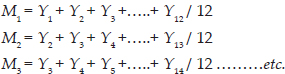
This is sequential manner for each points of time t. In this fashion, a 12 month centered moving average removes a large part of fluctuation due to the seasonal effects so that what remains is mainly attributable to other sources viz., long term effects Tt,, cyclical effect Ct and the irregular variation It wwhich is due to random causes is also minimized by the process of smoothing out effect. Thus, this affords a means of not only estimating TC effect but also estimating seasonal components. In the next step of computing the seasonal index, the original series is divided by the centered moving average. This gives the first estimate of seasonal component St..
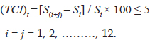
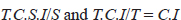
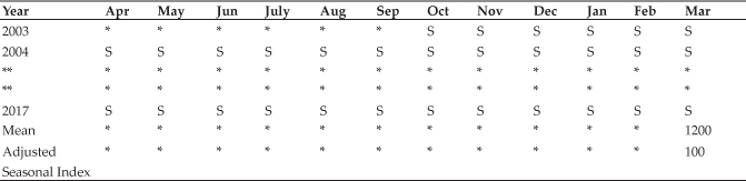
It is always expressed in terms of percentages. In this process, we do not have moving average for the first six and last six months. These seasonal components are next arranged month-wise for each year (Table 1). The last row in the Table 1 give estimates of seasonal index for the 12 months adjusted for their total to 1200 or averaged to 100. The last row in the Table. 1 gives the first estimates of seasonal variations. In order to obtain a better estimate i.e., stabilized seasonal indices we need to employ an interactive process as under. The original observation (Yt) is divided by corresponding (St)) value and then obtain the residual (TCI)t corresponding to time point t.
The residual series (TCI)t thus obtained is subjected to the same process of determining 12 month centered averages as done earlier to obtain better estimates for trend cycle effect viz., (TC)t. These revised estimates are next employed as above to generate a revised set of seasonal indices by dividing each observation (Yt) by the corresponding (TC)t value. This will lead to revise estimates of seasonal indices (St) as second interactive ones.
This interactive process is separately employed until stabilized seasonal indices are obtained i.e., two successive seasonal indices do not differ by more than five per cent.
Where adjusted
Seasonal indices = Seasonal indices × correction factor
and
Correction factor = 1200 / Sum of seasonal indices
Cyclical movements
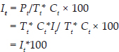
Cyclical variations are long term oscillatory movements with duration of greater than one year. The most commonly used method for estimating cyclical movement of time series is the residual method by eliminating the seasonal variation and trend. This is accomplished by dividing (Yt)) by corresponding (S) for time 'if
Symbolically,
Irregular variations: It was estimated as residual component by using the estimates of model prices and cyclical components.
The details of ARIMA forecasting model are as follows:
Auto Regressive Integrated Moving Average (ARIMA) Model
Introduced by Box and Jenkins (1976), the ARIMA model has been one of the most popular approaches for forecasting. The ARIMA model is basically a data oriented approach that is adopted from the structure of the data itself. In an ARIMA model, the estimated value of a variable is supposed to be a linear combination of the past values and the past errors. Generally a time series can be modelled as a combination of past values and errors, which can be denoted as ARIMA (p,d,q) which is expressed in the following form
Table 1: Average of percentage centered 12 months moving average and computation of seasonal index for observation
where Yt and et are the actual values and random error at time t, respectively, Φi (i = 1,2,....., p) and θj (j = 1,2,...., q) are model parameters, p and q are integers and often referred to as orders of autoregressive and moving average polynomials respectively. Random errors are assumed to be independently and identically distributed with mean zero and constant variance. Similarly, a seasonal model is represented by ARIMA (p, d, q) × (P, D, Q), where P is the number of seasonal autoregressive (SAR) terms, D is the number of seasonal differences and Q is the number of seasonal moving average (SMA) terms. Basically this method has four steps identification of the model, estimating the parameters, diagnostic checking and forecasting
RESULTS AND DISCUSSION
The results revealed that there was an increasing trend in onion prices in Kurnool market for the study period. The trend equation estimated for the present study was 264.39 + 6.22*t and graphically shown in Fig. 1. The annual increase in prices of onion in Kurnool market was observed to be ₹ 6.22 per quintal. Areef et al. (2019) revealed that the annual increase in prices of onion in Bangalore market was ₹ 6.92 per quintal for the period from Jan-2003 to Dec-2017 and it was found to be statistically significant. In order to analyse the seasonal variation in onion prices in the Kurnool market, seasonal indices were computed by adopting 12 months centered moving average method. The results (Table 2 and Fig. 2) revealed that the highest seasonal index was observed in August, followed by November and July as the indices stood at 140.80, 121.31 and 117.07 respectively. Lowest seasonal index was recorded in May with 62.72. The cyclical and irregular fluctuations in onion prices were graphically shown in Fig. 3 and Fig. 4 respectively. A definite periodic fluctuations were not identified in Kurnool market which was revealed by the absence of price cycles.
Table 2: Seasonal indices (%) in prices of onion in Kurnool market
For forecasting onion prices in Kurnool market, ARIMA model was used after transforming the variable under forecasting into a stationary series. The stationary series is the one whose values vary over time only around a constant mean and constant variance. Identification of the model was concerned with deciding the appropriate values of (p,d,q) (P,D,Q). It was done by observing Auto Correlation Function (ACF) and Partial Auto Correlation Function (PACF) values (Fig. 5). The Auto Correlation Function helps in choosing the appropriate values for ordering of moving average terms (MA) and Partial Auto-Correlation Function for those autoregressive terms (AR).
Table 3: Residual analysis of monthly prices of onion
ARIMA model was estimated after transforming the variables under study into stationary series through computation of either seasonal or non-seasonal or both, order of differencing. Based on the maximum R-Square, minimum MAPE (Mean Absolute Percentage Error), RMSE (Root Mean Square Error) and MAE (Mean Absolute Error) the model (1,1,1) (1,1,1) was found to be fit the data and suitable to forecast future prices in Kurnool market (Table 3).
Fig. 1 : Trends in prices of onion in Kurnool market
Fig. 2 : Seasonal indices of onion prices in Kurnool market
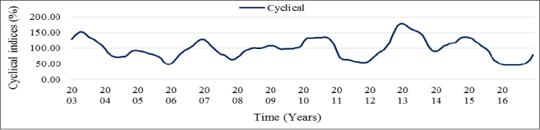
Fig. 3: Cyclical indices of onion prices in Kurnool market
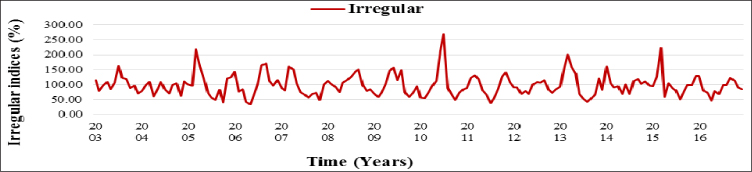
Fig. 4: Irregular indices of onion prices in Kurnool market
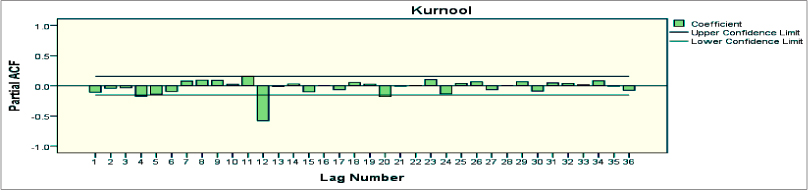
Fig. 5 : Autocorrelation and Partial Autocorrelation coefficients of onion prices in Kurnool market
Table 4: Conditional least square estimates of onion prices
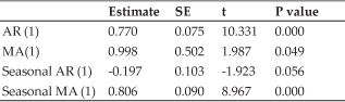
The parameters of the tentatively identified model were estimated and are presented in Table 4. The autocorrelation and partial autocorrelations of various orders of the residuals of ARIMA (1,1,1) (1.1,1) up to 36 lags were computed and are shown in Fig. 6. The figures showed that, the autocorrelation at lag 15 and 36 and partial autocorrelation functions at lag 15 and 20 were significantly different from zero and fell slightly outside the 95 per cent confidence interval, which indicated the presence of white noise error in the residuals.
Table 5: Ex-ante and Ex-post forecast of monthly prices of onion
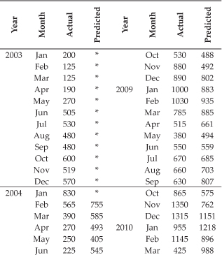
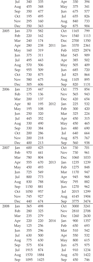
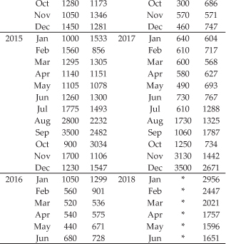
Hence, except for lag 15, 20 and 36 autocorrelation was absent in the residuals. This showed that the selected ARIMA model was appropriate for forecasting the price of onion during the period under study. Both ex-ante and ex-post forecasting were done and it was compared with actual observations. The prices were forecasted up to June, 2018. The results of ex-ante and ex-post forecasted prices are presented in Table 5 and illustrated in Fig. 7. The forecast are also depicted that there is narrow variations in between the actual and forecasted values of prices of onion in the Kurnool market. According to the forecasts the price of onion would be ranging from ' 2956 to ' 1651 per quintal for the months from January to June 2018.
CONCLUSION
Reliable price forecast model enable the government to make appropriate decisions in advance like procurement, regulating export & imports and possibility of check on trader hoardings. The price seasonal indices and forecasted price information was more important for the farmer to selection of crop varieties, allocation of scarce inputs under different crops and adjusting the sowing & harvesting dates to get remunerative prices in a more rational way.
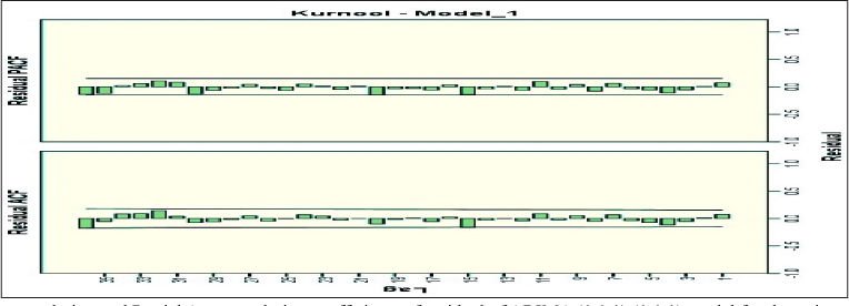
Fig. 6 : Autocorrelation and Partial Autocorrelation coefficients of residual of ARIMA (1,1,1) (1,1,1) model for the onion prices
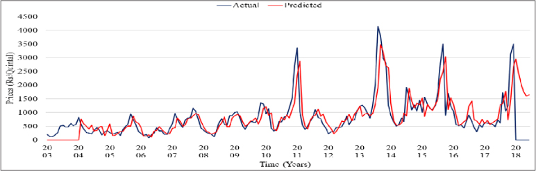
Fig. 7: Ex-ante and Ex-post forecast of monthly prices of onion in Kumool market
REFERENCES
Anonymous. 2018. National Horticultural Board, Database 2018, National Horticulture Board, Ministry of Agriculture and Farmer Welfare, Government of India.
Areef, M., Rajeswari, S., Vani, N. and Naidu, G.M. 2019. A study on price behaviour of onion in Bangalore market of Karnataka, India. The Andhra Agricultural Journal, 66 : 37-41.
Bhardwaj, S.P., Paul Ranjith Kumar, Singh, D.R. and Singh, K.N. 2014. An empirical investigation of ARIMA and GARCH models in agricultural price forecasting. Economic Affairs, 59 : 415-428.
Box, G.E.P. and Jenkins, G.M. 1976. Time series analysis: Forecasting and control, Second Edition, Holden Day.
Chahal, S.S., Singla, R. and Kataria, P. 2004. Marketing efficiency and price behaviour of green peas in Punjab. Indian Journal of Agricultural Marketing, 18 : 115-128.
Chandran, K.P. and Pandey, N.K. 2007. Potato price forecasting using seasonal ARIMA approach. Potato Journal, 34 : 1-2.
Chengappa, P.G., Manjunatha, A.V., Dimble, V. and Shah, K. 2012. Competitive assessment of onion markets in India. Institute for Social and Economic Change, Report for Competition Commission of India, Government of India.
Darekar, A.S., Datarkar, S.B. and Hile, R.B. 2015. Forecasting the prices of onion in Lasalgaon market of western Maharashtra. International conference on recent research Development in Environment, Social Sciences and Humanities,(conference special). 75-81.
Darekar, A.S., Pokharkar, V.G. and Yadav, D.B. 2016. Onion price forecasting in Yeola market of Western Maharashtra using ARIMA technique. International Journal of Advanced Biological Research, 6 : 551-552.
Darekar, A. and Reddy, A.A. 2017. Cotton price forecasting in major producing states. Economic Affairs, 62 : 373-378.
Devi, I.B., Srikala, M. and Ananda, T. 2016. Price behaviour of chillies in Guntur market of Andhra Pradesh, India. Indian Journal of Agricultural Research, 50 : 471-474.
Devi, I.B., Ram, P.R., Lavanya, T. and Vandana, S. 2011. Forecasting of prices of sunflower and groundnut in Andhra Pradesh- An application of ARIMA model. The Andhra Agricultural Journal, 58 : 368-370.
Guha, B. and Bandyopadhyay, G. 2016. Gold price forecasting using ARIMA model. Journal of Advanced Management Science, 4 : 117-121.
Kumari, R.V., Panasa, V., Gundu, R. and Kaviraju, S. 2017. Price behaviour and forecasting of cotton in Telangana. International Journal of Pure and Applied Biosciences, 5 : 863-871.
Majid, R. and Mir, S.A. 2018. Advances in statistical forecasting methods: An overview. Economic Affairs, 63: 815-831.
Markidakis, S. and Hibbon, M. 1979. Accuracy of forecasting: An empirical investigation. Journal of Royal Statistical Society of Australia, 142: 7-145.
Meera and Sharma, H. 2016. Trend and seasonal analysis of wheat in selected market of Sriganganagar district. Economic Affairs, 61: 127-134.
Sangeeta, S. 2004. Marketing of onion in Maharashtra. Indian Journal of Agricultural Marketing, 4 : 45- 50.
Sangsefidi, S.J., Moghadasi, R., Yazdani, S. and Nejad, M. 2015. Forecasting the prices of agricultural products in Iran with ARIMA and ARCH models. International journal of Advanced and Applied Sciences, 2 : 54-57.
Saxena, R. and Chand, R. 2017. Understanding the Recurring Onion Price Shocks: Revelations from Production-Trade- Price Linkages. ICAR-National Institute of Agricultural Economics and Policy Research (NIAP), New Delhi. Policy Paper 33.
Sharma, H. 2015. Applicability of ARIMA models in wholesale wheat market of Rajasthan: An investigation. Economic Affairs, 60: 687- 691.
Singh, D.K., Pynbianglang, K. and Pandey, N.K. 2017. Market arrival and price behaviour of potato in Agra district of Uttar Pradesh. Economic Affairs, 62: 341-345.
Srikala, M., Devi, I.B., Rajeswari, S., Naidu, G.M. and Prasad, S.V. 2018. Application of Time Series Models for Forecasting of Paddy Prices in Nizamabad Market (Telangana). Agricultural Situation in India, 74: 41-46.
Takle, S.R. 2002. Behaviour of market arrivals and prices of rabi jowar in Marathwada. Indian Journal of Agricultural Marketing, 16 : 73-75.
Vasudev, S. 2015. A study on the price instability and price behaviour of rice in Andhra Pradesh. Indian Journal of Agricultural Marketing, 29 : 26-32.
Vinayak, N.J. and Patil, B.L. 2015. Onion price forecasting in Hubli market of northern Karnataka using ARIMA technique. Karnataka Journal of Agricultural Science, 28 : 228-231.